neural network
- References :
- Done Reading:
- Reading:
- Tom Mitchell Lectures slides of chapter 4
- Tom Mitchell, Machine Learning Chapter 4
- To Read:
- Questions :
Biological Motivation
- Mimicing human brain
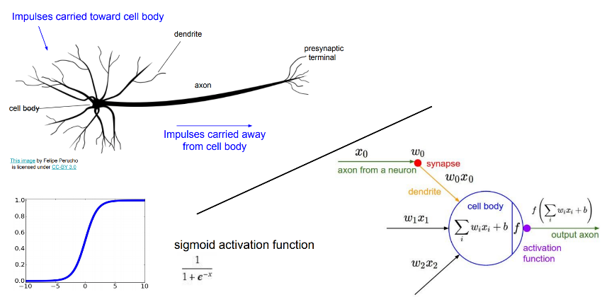
Figure 1: biological neuron vs aritifical neuron from this post
- properties that match with the human brain
- Many neuron like threshold switching units
- Many weighted interconnections among units
- Highly parallel, distributed process
- Emphasis on tuning weights automatically
Representations
- The ANNs can graphs be with many types of structures:
- acyclic or cyclic
- directed or undirected
- The backprop algorithm assumes ANN to have structure that corresponds to a directed graph, and possibly containing cyclees.
- Practical applications involves acyclic feed forward network structure for ANN
When is Neural Network suitable ?
- Instances are represented by many attribute value pairs
- has high dimensions
- The target function output may be
- discrete-valued,
- real-valued
- or a vector of several real or discrete valued attributes
- The training examples may contain noises
- Long training times are acceptable
- Fast evaluation of the learned target function may be required.
- The ability to understand the learned target function is not important
ALVINN System
- Autonomous Land Vehicle In a Neural Network
- 30 * 32 Sensor input retina as input vector
- outputs vector of 30 attributes [ gives directions]
A perceptron is a simple neural network
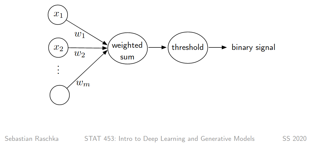
Figure 2: from Sebastian Raschka lectures
Gradient Descent And the Delta Rule
- To overcome the problem of failing to coverge on a non linearly separable data a training rule delta rule was designed.
- delta rule uses gradient descent to search the hypothesis space \(H\) to find the best weights for our training examples.
- Space \(H\) of candidate hypotheses is
- \(H = \{ \overrightarrow{w} | \overrightarrow{w} \in \Re^{n+1} \}\)
- Space \(H\) of candidate hypotheses is
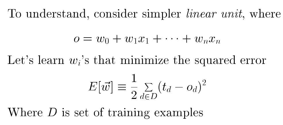
Figure 3: Error as function of w, from Tom Mitchell Lectures
- \(d\) is a training example at an instance
- \(t_{d}\) is target output
- \(o_{d}\) is output from linear unit, unthresholded
- for perceptron \(o_{d} = sgn(\overrightarrow{w}.\overrightarrow{x})\), where,
- \( sgn(y) = \begin{cases} 1 & \text{if y > 0} \\ -1 & \text{otherwise} \end{cases} \)
- for perceptron \(o_{d} = sgn(\overrightarrow{w}.\overrightarrow{x})\), where,
- \(E\) is the Error as a function of \(\overrightarrow{w}\)
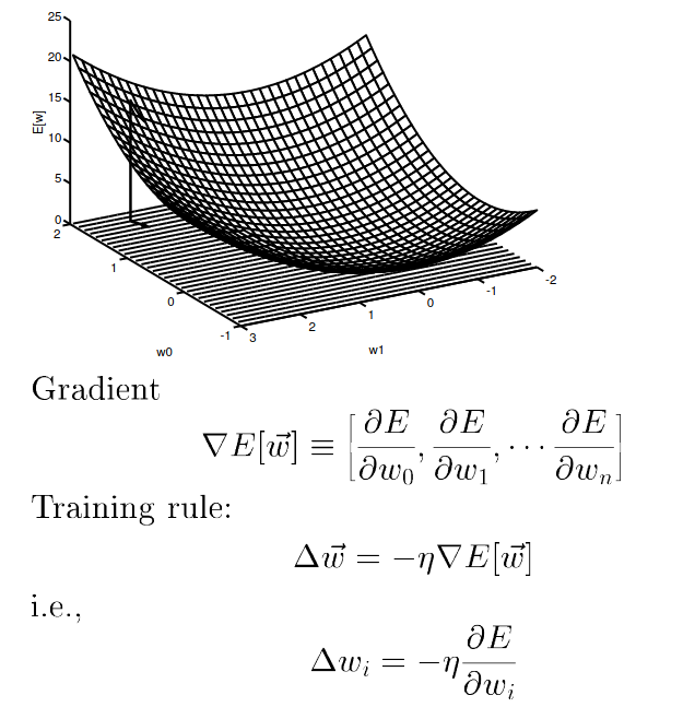
Figure 4: Gradient Descent Rule, from Tom Mitchell Lectures
- \( \nabla E(\overrightarrow{w}) \)
- is called gradient of E with respect to \(\overrightarrow{w}\)
- is a vector
- As a vector in a weight space, the gradient specifies the direction that produces the steepes increase in E
- So the negative of this vector gives the direction of steepest decrease, \( (-\nabla E(\overrightarrow{w})) \)
- We look for steepest decrease because we want to move the weight vector in the direction that decreases E.
For derivative of error(E) w.r.t \(i_{th}\) weight
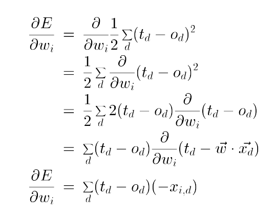
Figure 5: Gradient Descent, E w.r.t wi, from Tom Mitchell Lectures
- \( \Delta{w_{i}} = \eta \sum_{d \in D} (t_{d} - o_{d}) x_{id} \)
- Here i represents the ith feature/component
Algorithm
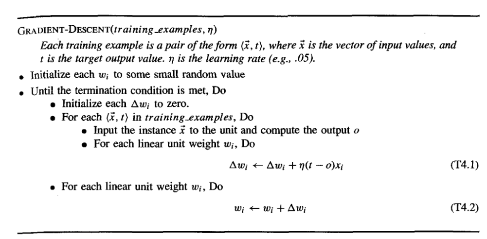
Figure 6: Gradient Descent Algo , from Tom Mitchell Book
- Computes weight updates after summing over all the training examples in D
About the Learning Rate and Gradient Descent
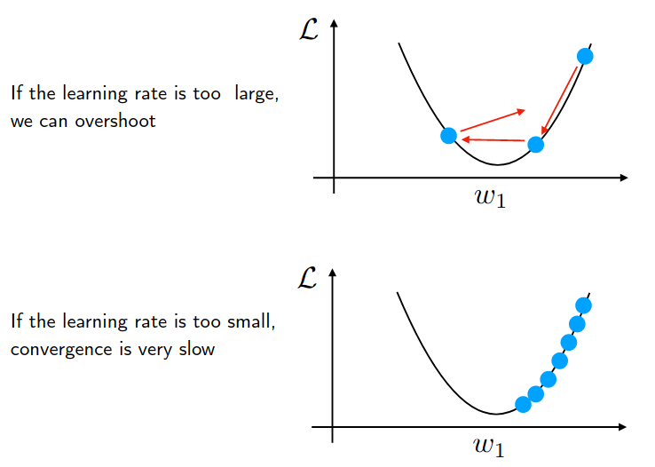
Figure 7: from Sebastian Raschka letcures
Stochastic Approximation to gradient descent
The key practical difficulties in applying gradient descent are
- converging to a local minimum can sometimes be quite slow (i.e.,it can require many thousands of gradient descent steps), and
- if there are multiple local minima in the error surface, then there is no guarantee that the procedure will find the global minimum.
For such problem stochastic (random) gradient descent (incremental gradient descent) was introduced.
The idea behind stochastic gradient descent is to approximate this gradient descent search by updating weights incrementally, following the calculation of the error for each individual example.
To modify the gradient descent algorithm shown in Figure 6 to implement this stochastic approximation, Equation (T4.2) is simply deleted and Equation (T4.1) replaced by,
- \( w_{i} \leftarrow w_{i} + \eta (t - o) x_{i} \)
here, \( \Delta w_{i} = \eta (t - o) x_{i} \)
- This is Delta rule, also Known as
- Adaline Rule
- LMS (least mean square)
- Widrow-Hoff (inventors of the rule)
- This is Delta rule, also Known as
Gradient Descent vs Stochastic Gradient Descent
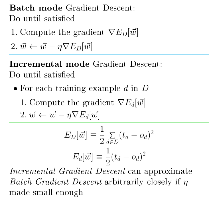
Figure 8: GD vs SGD, from Tom Mitchell Lectures
- In standard gradient descent, the error is summed over all examples before updating weights, whereas in stochastic gradient descent weights are updated upon examining each training example.
- Summing over multiple examples in standard gradient descent requires more computation per weight update step. On the other hand, because it uses the true gradient, standard gradient descent is often used with a larger step size per weight update than stochastic gradient descent.
- In cases where there are multiple local minima with respect to \(E(\overrightarrow{w})\), stochastic gradient descent can sometimes avoid falling into these local minima because it uses the various \(\Delta E_{d}(\overrightarrow{w})\) rather than \(\Delta E(\overrightarrow{w})\) to guide its search.
Delta rule vs Perceptron rule
- The difference between these two training rules is reflected in different convergence properties.
- The perceptron training rule converges after a finite number of iterations to a hypothesis that perfectly classifies the training data, provided the training examples are linearly separable.
- The delta rule converges only asymptotically toward the minimum error hypothesis, possibly requiring unbounded time, but converges regardless of whether the training data are linearly separable.
- delta rule can be easily extended to multilayer neural network
Multilayer Networks
- Capable of expressing a rich variety of non linear decision
Differentiable Threshold Unit
- We need to introduced units which can help represents non linearity
- Perceptron unit can be used but is discontinuous threshold makes it undifferentiable.
Sigmoid unit
- output is a non linear function of its inputs and is differentiable threshold function
- Tanh is also used in place of the sigmoid
- error gradient with sigmoid
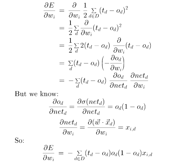
Figure 9: error gradient with sigmoid unit, from Tom Mitchell Lectures
Backpropagation Algorithm
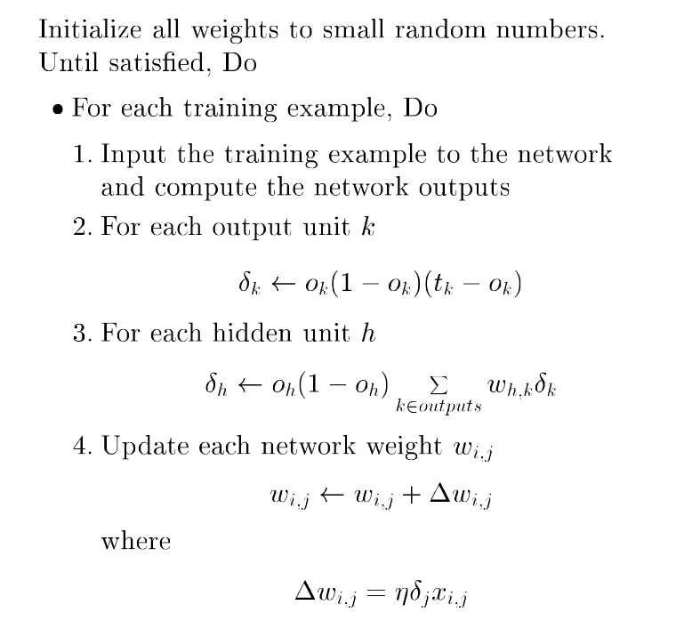
Figure 10: error gradient with sigmoid unit, from Tom Mitchell Lectures
\(\sum_{k \in outputs} w_{hk} \delta_{k}\) = error term for hidden unit h
- since training examples provide target values \(t_{k}\) only for network outputs, no target values are directly available to indicate the error of hidden units’ values.
- \(w_{hk}\) is weight form hidden unit \(h\) to output unit \(k\)
- This weight characterizes the degree to which hidden unit h is “responsible for” the error in output unit k.
Easily generalizes to arbitary directed graphs
It is peformed only during training
Adding momentum
making the weight update on the nth iteration depend partially on the update that occurred during the (n - 1)th iteration, as
- \(\Delta w_{ji}(n) = \eta \delta_{j} x_{ji} + \alpha \Delta wji(n - 1)\)
Here \(\Delta w_{ji}(n)\) is the weight update performed during the nth iteration through the main loop of the algorithm, and \(0 < \alpha < 1\) is a constant called the momentum.
- \( \eta \delta_{j} x_{ji} \sim \eta \frac{\partial E}{\partial w_{i}} \)
Momentum can sometimes carry the gradient descent procedure through narrow local minima (though in principle it can also carry it through narrow global minima into other local minima!).
For Convergence
- Train multiple nets with different initial weights
- Add momentum
- Stochastic Gradient descent
Representation power of feedforward networks
- Boolean functions
- Continuous functions
- Arbitrary Functions
Hypothesis space search and Inductive Bias
- Hypothesis space is continuous, in contrast to the hypothesis spaces of decision tree learning and other methods based on discrete representations.
- Hypothesis space is the n-dimensional Euclidean space of the n network weights. i.e For Backpropagation, every possible assignment of network weights represents a syntactically distinct hypothesis that in principle can be considered by the learner.
- Inductive Bias
- One can roughly characterize it as smooth interpolation between data points.
Other concepts
Generalization, Overfitting and Stopping Criterion
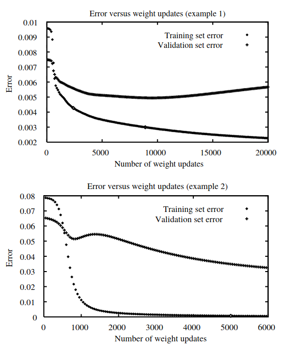
Figure 11: overfiiting , from Tom Mitchell Lectures
- In first plot, generalization accuracy measured over the validation examples first decreases, then increases, even as the error over the training examples continues to decrease.
- this occurs because the weights are being tuned to fit oddity of the training examples that are not representative of the general distribution of examples.
- Notice in the second plot, one must be careful to not stop training too soon when the validation set error begins to increase.
- Overfitting tend to occur during later iterations, but not during earlier iterations
- As training proceeds, some weights begin to grow in order to reduce the error over the training data, and the complexity of the learned decision surface increases.
- How many weight-tuning iterations should the algorithm perform?
- it should use the number of iterations that produces the lowest error over the validation set.
- We can try Early Stopping
- K-fold cross-validation approach is sometimes used, in which cross validation is performed K different times, each time using a different partitioning of the data into training(k-1 part of data) and validation sets(1 part of data) , and the results are then averaged.
Weight decay
- One of the solutions to solve overfitting
- Decrease each weight by some small factor during each iteration.
- This is equivalent to modifying the definition of E to include a penalty term corresponding to the total magnitude of the network weights.
Alternative Error
Penalty term for weight magnitude
- To solve overfitting as mentioned in Weight decay
- Add a term to E that increases with the magnitude of the weight vector.
- This causes the gradient descent search to seek weight vectors with small magnitudes, thereby reducing the risk of overfitting.
- \( E(\overrightarrow{w}) = \frac{1}{2} \sum_{d \in D} \sum_{k \in outputs} (t_{kd} - o_{kd})^2 + \gamma \sum_{i,j} w_{ji} ^ 2 \)
- \( \sum_{i,j} w_{ji} ^2 \) is the regularization term
- \(\gamma\) controls the importance of the regularization term
Train on target slopes as well as values
- Adding a term for errors in the slope, or derivative of the target function.
- \( E(\overrightarrow{w}) = \frac{1}{2} \sum_{d \in D} \sum_{k \in outputs} [ (t_{kd} - o_{kd})^2 + \mu \sum_{j \in inputs} (\frac{\partial t_{kd}}{\partial x_{d}^j} - \frac{\partial o_{kd}}{\partial x_{d}^j} ) ^ 2 ] \)
- \(\frac{\partial t_{kd}}{\partial x_{d}^j}\) describes how the target output value should vary with a change in the input.
- \(\frac{\partial o_{kd}}{\partial x_{d}^j}\) describes how the observed value should vary with a change in the input.
- The constant \(\mu\) determines the relative weight placed on fitting the training values versus thetraining derivatives.
Minimizing the cross entropy of the network with respect to the target values.
- \( - \sum_{d \in D} t_{d} log(o_{d}) + (1 - t_{d})(1 - log(o_{d})) \)
Recurrent Networks(RNN)
Python implementation
Trying W.x in vectorized form
import numpy as np

x = [[1.,2.,3.]]
x_np = np.array(x)
print(x_np.shape)

w = [[0.1,0.2,0.3]]
w_np = np.array(w)

print(w_np.shape)
# Passing SIngle Point
z = x_np[0].dot(w_np[0])
print(z.shape)
print(f"Single datapoint, z = {z.sum()}")
# Passing Batch
z = w_np.dot(x_np.T)
print(z.shape)
print(f"Batch format, z = {z.sum()}")
(1, 3)
(1, 3)
()
Single datapoint, z = 1.4
(1, 1)
Batch format, z = 1.4