image filtering
- References :
- Done Reading
- Reading
- To read:
- Questions :
Modify image pixels based on some function of a local neighbourhood of each pixel.
Why filter a image
- To sharpen,
- smooth,
- intensify or
- enhance a imag
Linear filters
Output pixel’s value is determined as a weighted sum of input pixel values within a small neighborhood N,
- \(g(i, j) = \sum_{k,l}{f(i + k, j + l)h(k, l)}\)
The entries in the weight kernel or mask h(k, l) are often called the filter coefficients.
The above correlation operator can be more compactly notated as
- \(g = f \otimes h\)
Correlation can be used for Template Matching
Variant of above formula is
- \(g(i, j) = \sum_{k,l}{f(i - k, j - l)h(k, l)}\)
where the sign of the offsets in f has been reversed, This is called the convolution operator,
- \(g = f \ast h\)
- Equivalent to flip the filter in both directions (bottom to top, right to left) and apply cross-correlation
h is called the impulse response function.
Difference between convolution and correlation operation
- h, convolved with an impulse signal, δ(i, j) (an image that is 0 everywhere except at the origin) reproduces itself, h * δ = h, whereas correlation produces the reflected signal.
Gaussian Filter/Blur
- good for denoising normally/gaussian distributed noise
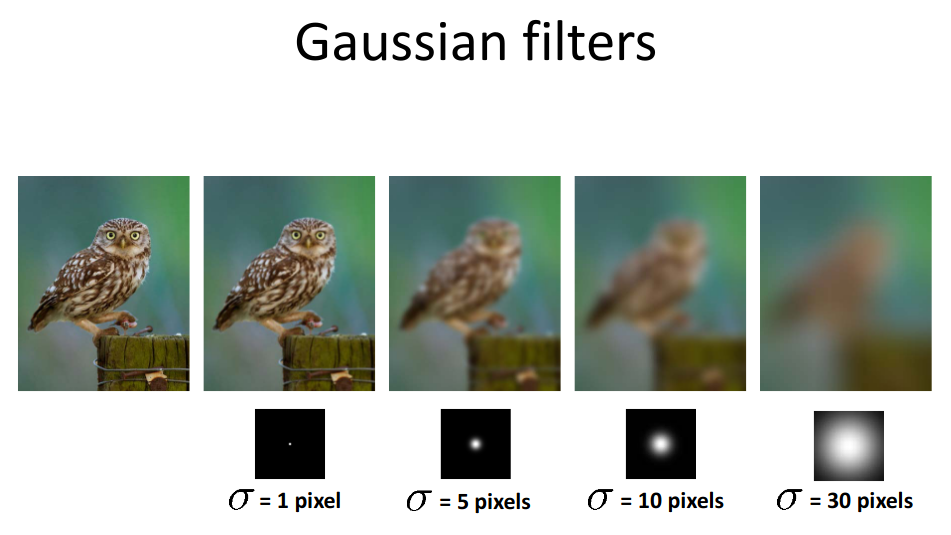
Figure 1: from cornell CV lecture
# img should be float so that operation works properly
g_img1 = cv2.GaussianBlur(img, (3,3), 0, borderType=cv2.BORDER_CONSTANT)

g_img2 = skimage.filters.gaussian(img, sigma=1, mode='constant', cval=0.0)
Non linear filters
median filter
- for denoising the salt and pepper noise
- Replace each pixel with MEDIAN value of all pixels in neighbourhood
- median calculation over the given filter size
- Properties:
- Non-linear
- Does not spread noise
- Can remove spike noise
- Robust to outliers, but not good for Gaussian noise
![Figure 2: from nptel [IIT Madras] CV lecture slide](/blogs/ox-hugo/2021-05-29_18-01-48_screenshot.png)
Figure 2: from nptel [IIT Madras] CV lecture slide
from skimage.filters import median
from skimage.morphology import disk

median_cv = cv2.medianBlur(img, 3)

median_skimage = median(img, disk(3), mode='constant', cval=0.0)
entropy filter
The entropy filter can detect subtle variations in the local gray level distribution. It is usually used to classify textures, a certain texture might have a certain entropy as certain patterns repeat themselves in approximately certain ways.
from skimage.filters.rank import entropy
from skimage.morphology import disk
entropy_img = entropy(img, disk(3))
Bilateral filter
- Edge perserving denoising filter.
- Noise removal comes at expense of image blurring at edges.
- Simple, non-linear edge-preserving smoothing.
- Reject(in a soft manner) pixels whose values differ too much from the central pixel value(outlier rejection).
- Output pixel value is weighted combination of neighboring pixel values: \(g(i,j) = \frac{\sum_{k,l}f(k,l) w(i,j,k,l)}{\sum_{k,l}w(i,j,k,l)}\)
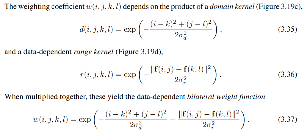
Figure 3: from szeliski book, chapter 3
- \(\sigma_{d}\) controls influence of the distant pixels.
- \(\sigma_{r}\) controls the influence of pixels with intensity value different from center pixel intensity.
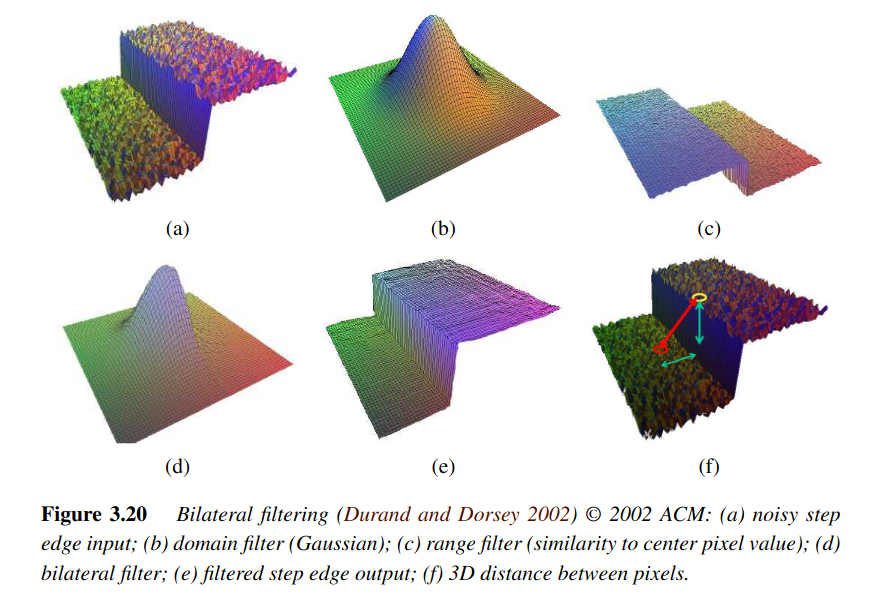
Figure 4: from szeliski book, chapter 3
bilateral_img_cv = cv2.bilateralFilter(image,
                                    d=5,
                                    sigmaColor=20,
                                    sigmaSpace=100,
                                    borderType=cv2.BORDER_CONSTANT)

from skimage.restoration import denoise_bilateral
bilateral_img_sk  = denoise_bilateral(image,
                                      win_size,
                                      sigma_color=0.05,
                                      sigma_spatial=15,
                                      mode='constant',
                                      cval=0,
                                      multichannel=False)
Non-local Means filter
- Estimated value is the weighted average of all pixels in the image but, the family of weights depend on the similarity between the pixels i and j.
- Similar pixel neighborhoods give larger weights.
- The non-local means algorithm replaces the value of a pixel by an average of a selection of other pixels values: small patches centered on the other pixels are compared to the patch centered on the pixel of interest, and the average is performed only for pixels that have patches close to the current patch. As a result, this algorithm can restore well textures, that would be blurred by other denoising algorithm.
"""
https://scikit-image.org/docs/dev/auto_examples/filters/plot_nonlocal_means.html
"""
from skimage.restoration import denoise_nl_means, estimate_sigma

sigma_est = np.mean(estimate_sigma(img, multichannel=False))
denoise_img = denoise_nl_means(img,
                               h=1.0*sigma_est,
                               fast_mode=True,
                               patch_size=5,
                               patch_distance=3,
                               multichannel=False)
Total Variation filter
- Signal with excessive spurious(counterfeit) detail have high total variation
- Reducing the total variation of the signal, removes unwanted detail while preserving important details such as edges.
- The result of this filter is an image that has a minimal total variation norm, while being as close to the initial image as possible.
- The total variation is the L1 norm of the gradient of the image.
- good for normally/gaussian distributed noise
from skimage.restoration import denoise_tv_chambolle
denoise_img_tv = denoise_tv_chambolle(img,
                                  weight=0.1,
                                  eps=0.0002,
                                  n_iter_max=200,
                                  multichannel=True)
BM3D (Block Matching and 3D filtering)
- Collaborative filtering process
- Group of similar blocks extracted from the image.
- A block is grouped if its dissimilarity with a reference fragment falls below a specified threshold - block matching.
- All blocks in a group are then stacked together to form 3D cylinder- like shapes.
- Filtering is done on every block group.
- Linear transform is applied followed by wiener filtering, then transform is inverted to reproduce all filtered blocks.
- Image transformed back to its 2D form.
import bm3d
"""
 bm3d library is not well documented yet, but looking into source code....
 sigma_psd - noise standard deviation
 stage_arg: Determines whether to perform hard-thresholding or Wiener filtering.
 stage_arg = BM3DStages.HARD_THRESHOLDING or BM3DStages.ALL_STAGES (slow but powerful)
 All stages performs both hard thresholding and Wiener filtering.
"""
bm3d_denoised = dm3d.bm3d(noisy_img,
                          sigma_psd=0.2,
                          stage_arg=bm3d.BM3DStages.ALL_STAGES)
anisotropic diffusion
Unsharp Mask
- Sharped = Original Image + (Orginial - Gaussian Blurred Image) * Amount
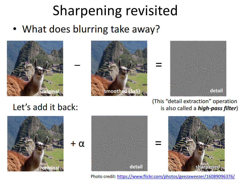
Figure 5: from cornell CV lecture
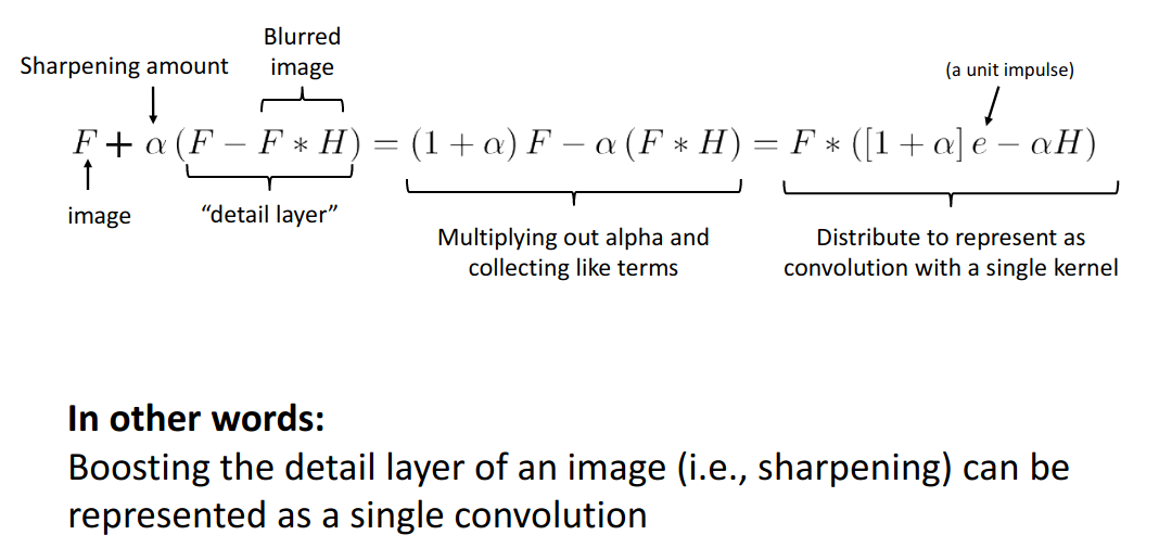
Figure 6: from cornell CV lecture
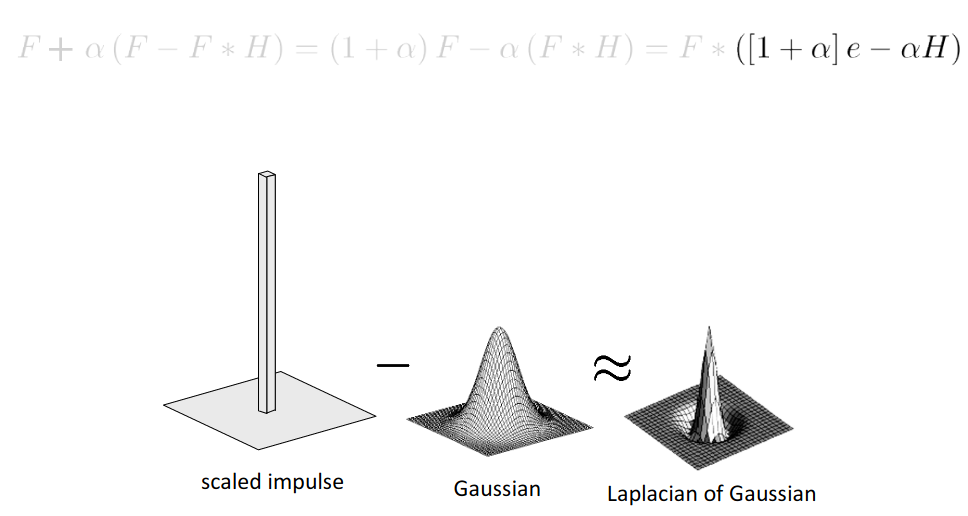
Figure 7: from cornell CV lecture
from skimage.filters import unsharp_mask
unsharped_img = unsharp_mask(img, radius=3, amount=1.0)
Edge Filters
Ridge filters
for detecting ridges in the image
In skimage
- meijering
- sato
- frangi
- hessian
from skimage.filters import meijering, sato, frangi, hessian
meijering_img = meijering(img)
sato_img  = sato(meijering)
frangi_img= frangi(img)
hessian_img = hessian(img)
Low and High Pass filters
Low-Pass Filters:
- Filters that allow low frequencies to pass through (block high frequencies).
- Example: Gaussian filter
High-Pass Filters:
- Filters that allow high frequencies to pass through (block low frequencies).
- Example: Edge filter
Discrete Fourier Transform
In python
import cv2
# img dtype should be checked so that operation works properly
# applying filter using opencv
convolved_image = cv2.filter2D(img, -1, kernel, borderType=cv2.BORDER_CONSTANT)