decision tree
References :
- Reading :
- Tom Mitchell Lectures slides of chapter 3
- Tom Mitchell, Machine Learning Chapter 3
- ID3 algorithm complete solution
- To Read :
- Reading :
Questions :
- Approximating discrete-valued fucntions
- robust to noisy data
- capable of learning disjunctive expressions
- search a completely expressive hypothesis space and thus avoid the difficulties of restricted hypothesis spaces.
Representation
- Decision trees classify instances by sorting them down the tree from the root to some leaf node
- each leaf node assigns a classification
- each interal node specifies a test of some attributes of the instances
- each branch descending from a node corresponds to one of the possible values of the attribute represented by that node.
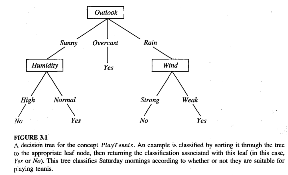
- For the instance <Outlook = Sunny, Temperature = Hot, Humidity = High, Wind=Strong>
- PlayTennis = no
- In general, decision trees represent a disjunction of conjunctions of constraints on the attribute values of instances.
- Each path from the tree root to a leaf corresponds to a conjunction of attribute tests, and the tree itself to a disjunction of these conjunctions.
When is Decision Tree suitable ?
- Instances are represented by many attribute value pairs.
- The target function output may be
- discrete-valued,
- with certain extension can be used for real-valued output
- The training examples may contain noises/errors
- Disjunctive descriptions may be required
- The training data may contain missing attribute values
ID3
- Basic algorithm for learning decision tree.
- “Which attribute should be tested at the root of the tree?”
- Which attribute to test at each node in the tree
entropy
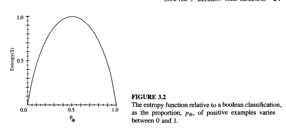
- Given a collection 5, containing positive and negative examples of some target concept, the entropy of S relative to this boolean classification is
- \( Entropy(S) = - p_{\oplus} log_2 p_{\oplus} - p_{\ominus} log_2 p_{\ominus} \)
- where, \(p_{\oplus}\) is the proportion of positive examples in S and,
- \(p_{\ominus}\) is the proportion of negative examples in S.
- Example,
- Entropy([9+, 5-]) = 0.940
- Entropy is
- 0 if all members of S belong to the same class.
- 1 when the collection contains an equal number of positive and negative examples.
- If the target attribute can take on c different values, then the entropy of S relative to this c-wise classification is defined as
- \( Entropy(S) = \sum_{i=1}^{c} - p_i log_2 p_i \) , where \(p_i\), is the proportion of S belonging to class i.
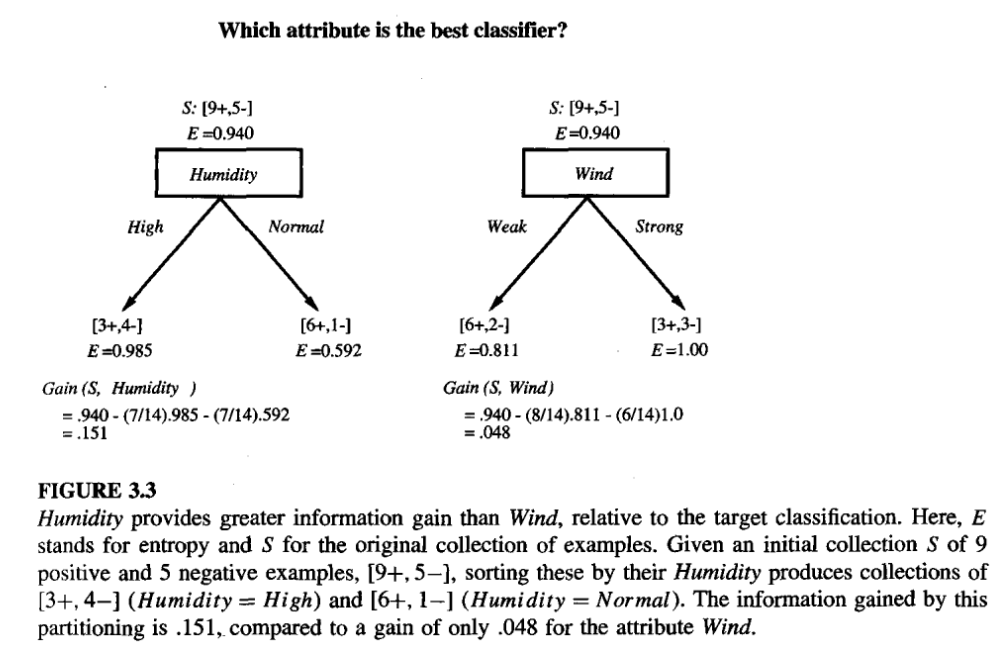
Information gain
- measures how well a given attribute separates the training examples according to their target classification.
- ID3 uses it to select attributes among the candidate attributes at each step while growing the tree.
- It is the expected reduction in the entropy caused by partitioning the examples based on the attributes
- the information gain, Gain(S, A) of an attribute A, relative to a collection of examples S, is defined as
- \( Gain(S,A) = Entropy(S) - \sum_{v \in Values(A)} \frac{|S_v|}{|S|} Entropy(S_v) \)
- where, Values(A) is the set of all possible values for attribute A,
- \(S_v\) is the subset of S for which attribute A has value v (i.e., \( S_v = \{s \in S|A(s) = v\}) \).
- the first term is just the entropy of the original collection S,
- and the second term is the expected value of the entropy after S is partitioned using attribute A.
- Gain(S, A) is
- the information provided about the target function value, given the value of some other attribute A.
- the number of bits saved when encoding the target value of an arbitrary member of S, by knowing the value of attribute A.
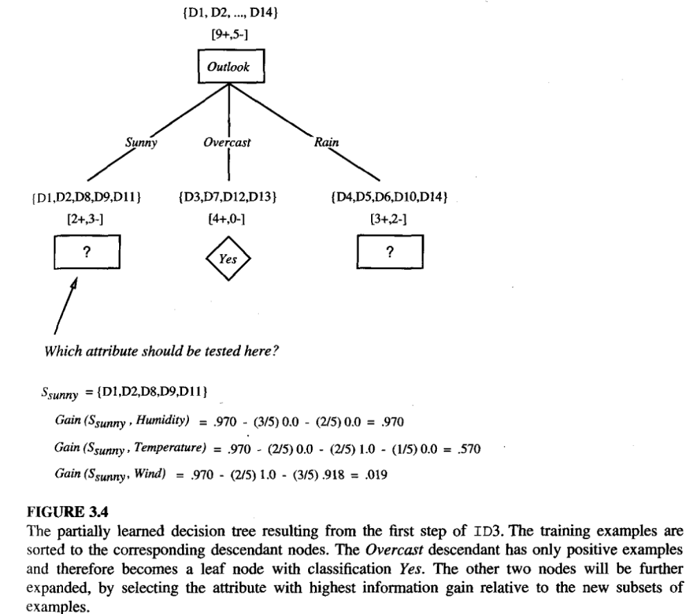
Illustrative Example
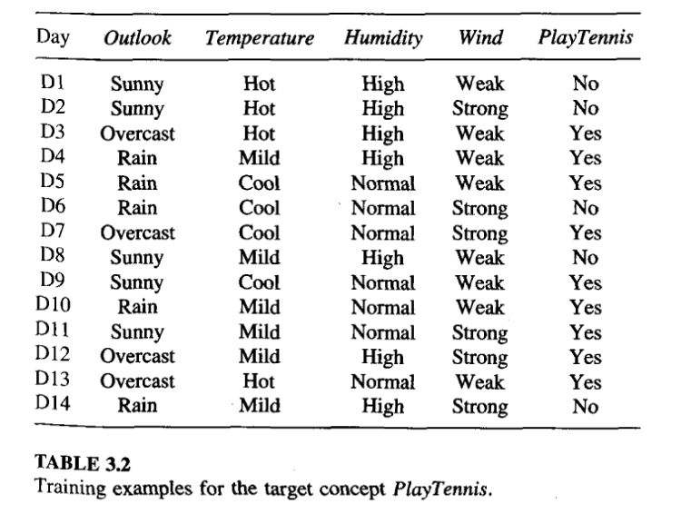
- The information gain values for all four attributes are
- Gain(S, Outlook) = 0.246
- Gain(S, Humidity) = 0.151
- Gain(S, Wind) = 0.048
- Gain(S, Temperature) = 0.029
- ID3 algorithm complete solution
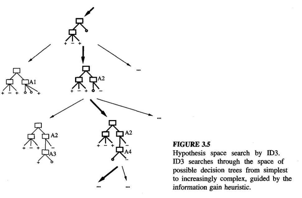
Hypothesis Space Search
- ID3 performs a simple-to-complex, hill-climbing search through hypothesis space,
- beginning with the empty tree,
- then considering progressively more elaborate hypotheses in search of decision tree that correctly classifies the training data.
- hill-climbing search is guided information gain measure.
Limitations and Capabilities of ID3
- ID3’s hypothesis space of all decision trees is a complete space of finite discrete-valued functions, relative to the available attributes.
- Thus, avoids one of the major risks of methods that search incomplete hypothesis spaces(such as methods that consider only conjunctive hypotheses): that the hypothesis space might not contain the target function.
- Maintains only a single current hypothesis as it searches through the space of decision trees.
- wheras, Candidate-Elimination Learning Algorithm, which maintains the set of all hypotheses consistent with the available training examples.
- it does not have the ability to determine how many alternative decision trees are consistent with the available training data,
- ID3 in its pure form performs no backtracking in its search.
- usually risks of hill-climbing search without backtracking: converging to locally optimal solutions that are not globally optimal.
- ID3 uses all training examples at each step in the search to make statistically based decisions regarding how to refine its current hypothesis.
- contrasts with methods that make decisions incrementally, based on individual training examples (e.g., Find-S or Candidate-Elimination Learning Algorithm)
- Advantage is that the resulting search is much less sensitive to errors in individual training examples.
Inductive Bias
the ID3 search strategy
- selects in favor of shorter trees over longer ones, and
- selects trees that place the attributes with highest information gain closest to the root.
Approximate inductive bias of ID3:
- Shorter trees are preferred over larger trees.
BFS-ID3, Breadth First Search for ID3
A closer approximation to the inductive bias of ID3:
- Shorter trees are preferred over longer trees. Trees that place high information gain attributes close to the root are preferred over those that do not.
Restriction and Preference Biases
- the inductive bias of
- ID3 follows from its search strategy,
- Candidate-Elimination algorithm follows from the definition of its search space.
- ID3 exhibits a purely preference bias(search bias), and
- A preference for certain hypotheses over others (e.g., for shorter hypotheses), with no hard restriction on the hypotheses thatcan be eventually enumerated.
- Candidate-Elimination purely restriction bias(language bias).
- Categorical restriction on the set of hypotheses considered.
- A preference bias is more desirable than a restriction bias,
- because it allows the learner to work within a complete hypothesis space that is assured to contain the unknown target function.
Why prefer Short Hypotheses
Occam’s razor
- Prefer the simplest hypothesis that fits the data.
- Why? (Argument in Favor)
- One argument is that because there are fewer short hypotheses than long ones, it is less likely that one will find a short hypothesis that coincidentally fits the training data.
- In contrast there are often many very complex hypotheses that fit the current training data but fail to generalize correctly to subsequent data.
- Argument Opposed
- There are many ways to define small sets of hypothesis
Issues
- Practical issues in learning decision trees :
- determining how deeply to grow the decision tree,
- handling continuous attributes,
- choosing an appropriate attribute selection measure,
- handling training data with missing attribute values,
- handling attributes with differing costs,
- and improving computational efficiency.
Avoiding overfitting the data
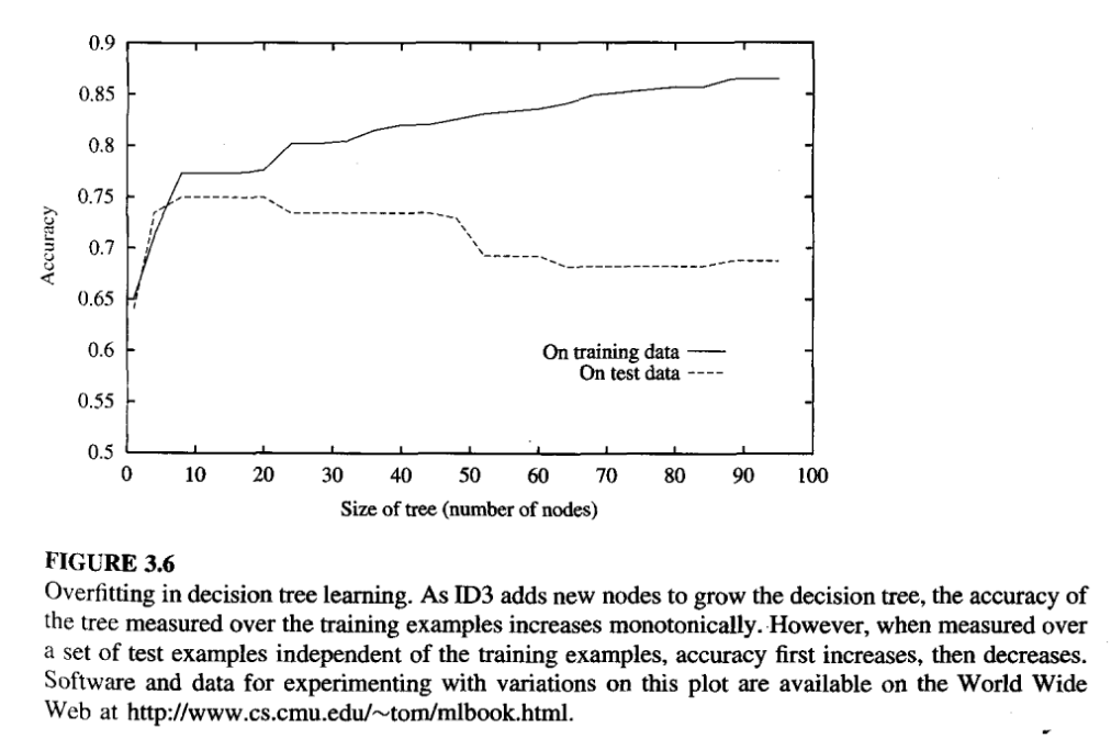
Overfitting
Given a hypothesis space H, a hypothesis \(h \in H\) is said to overfit the training data if there exists some alternative hypothesis \(h’ \in H\), such that h has smaller error than h’ over the training examples, but h’ has a smaller error than h over the entire distribution of instances.
\( error_{train}(h) < error_{train}(h’) \)
\( error_{D}(h) > error_{D}(h’) \)
This could be due to
- Random errors and noise in the data, or
- The number of training examples is too small to produce a representative sample of the true target function.
Approaches to avoid overfitting
Stop growing the tree earlier, before it reaches the point where it perfectly classifies the training data,
- stop growing when data split not statistically significant
- seems to be more direct but difficulty in the estimating precisely when to stop growing the tree.
Allow the tree to overfit the data, and then post-prune the tree.
- sucessful in practice
How to select “best” tree
Use a separate set of examples, distinct from the training examples, to evaluate the utility of post-pruning nodes from the tree.
- training and validation set approach.
Use all the available data for training, but apply a statistical test to estimate whether expanding (or pruning) a particular node is likely to produce an improvement beyond the training set.
- Quinlan(1986) uses a chi-square test to estimate whether further expanding a node is likely to improve performance over the entire instance distribution, or only on the current sample of training data.
Use an explicit measure of the complexity for encoding the training examples and the decision tree, halting growth of the tree when this encoding size is minimized.
- The Minimum Description Length principle,
- \( size(tree) + size(missclassifcations(tree)) \)
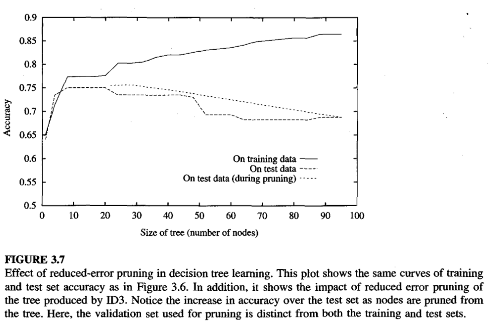
Pruning Approaches
Pruning by reducing the error
- reduced-error pruning (Quinlan 1987), consider each of the decision nodes in the tree to be candidates for pruning.
- Pruning a decision node consists of removing the subtree rooted at that node, making it a leaf node, and assigning it the most common classification of the training examples affiliated with that node.
- Nodes are removed only if the resulting pruned tree performs no worse than the original over the validation set.
- effect of any leaf node added due to coincidental regularities in the training set is likely to be pruned because these same coincidences are unlikely to occur in the validation set.
- Nodes are pruned iteratively, always choosing the node whose removal most increases the decision tree accuracy over the validation set.
- Pruning of nodes continues until further pruning is harmful (i.e., decreases accuracy of the tree over the validation set).
Rule Post Pruning
- by C4.5 (Quinlan 1993),
- Involves the following steps:
- Infer the decision tree from the training set, growing the tree until the training data is fit as well as possible and allowing overfitting to occur.
- Convert the learned tree into an equivalent set of rules by creating one rule for each path from the root node to a leaf node.
- Prune (generalize) each rule by removing any pre conditions that result in improving its estimated accuracy.
- Sort the pruned rules by their estimated accuracy, and consider them in this sequence when classifying subsequent instances.
- From figure of decision tree
- IF (outlook = Sunny) and (Humidity = High)
- THEN PlayTennis = No
- IF (outlook = Sunny) and (Humidity = Normal)
- THEN PlayTennis = Yes
- IF (outlook = Sunny) and (Humidity = High)
- Why convert tree to set of rules
- allows distinguishing among the different contexts in which a decision node is used.
- removes the distinction between attribute tests that occurnear the root of the tree and those that occur near the leaves.
- improves readability.
Incorporating Continuous-Valued Attributes
- Restriction is “the attributes tested in the decision nodes ofthe tree must also be discrete valued”.
- This restriction can be removed.
- dynamically defining new discrete-valued attributes that partition the continuous attribute value into a discrete set of intervals.
- In particular, for an attribute A that is continuous-valued, the algorithm can dynamically create a new boolean attribute \(A_c\) that is true if A < cand false otherwise.
- for the threshold c.
- pick a threshold, c, that produces the greatest Information gain.
- value of c that maximizes information gain must always lie at a boundary of sorted examples according to the continuous attribute(Fayyad 1991).
Alternative Measures for Selecting Atrributes
- gain ratio (Quinlan 1986).
- The gain ratio measure penalizes attributes having many value(Date = June 03 1996) attributes by incorporating a term, called split information, that is sensitive to how broadly and uniformly the attribute splits the data:
- \( SplitInformation(S, A) \equiv - \sum_{i=1}^{c} \frac{|S_i|}{|S|} log_2{\frac{|S_i|}{|S|}} \)
- where \(S_i\) through \(S_c\) are the c subsets of examples resulting from partitioning S by the c-valued attribute A.
- SplitInformation is actually the entropy of S with respect to the values of attribute A.
- The GainRatio measure is defined in terms of the earlier Gain measure, as well as this Splitlnformation, as follows
- \( GainRatio(S, A) \equiv \frac{Gain(S,A)}{SplitInformation(S,A)} \)
- SplitInformation term discourages the selection of attributes with many uniformly distributed values.
Handling Training Examples with Missing Attribute Values
- Use training example anywat, sort through tree
- If node n tests A, assign most commom value of A among other examples sorted to node n
- Assign most common value of A among other examples with same target value
- Assign probalility of \(p_i\) to each posssible value \(v_i\) of A
- assign fraction of \(p_i\) of example to each descendant in tree
- classify new example in similar fashion
Handling Attributes With Differing Costs
- prefer decision trees that use low-cost attributes where possible, relying on high-cost attributes only when needed to produce reliable classifications.
- Replace gain by
- Tan and Schlimmer(1990) and Tan(1993)
- \( \frac{Gain^2(S,A)}{Cost(A)} \)
- Can be applied to a robot perception task
- Nunez(1998)
- \( \frac{2^{Gain(S,A)} - 1}{(Cost(A) + 1)^w} \)
- where \( w \in [0,1] \) is a constant that determines the relative importance of cost versus information gain.
- Tan and Schlimmer(1990) and Tan(1993)