concept learning
- References :
- Reading:
- Tom Mitchell Lectures slides of chapter 2
- Tom Mitchell, Machine Learning Chapter 2
- To Read:
- Reading:
- Questions :
- Inferring boolean valued function from training examples of its input and outputs.
- A problem of searching through a predefined space of potential hypotheses for the hypothesis that best fits the training examples
Example
- Traget concept or function:
- Concept or function to be learned.
- For our example - “days on which “A” can enjoy water sport”, EnjoySport
- Denoted by \(c\)
- c can be any boolean valued function defined over the instances X; \( c : X \rightarrow \{ 0,1 \} \)
- Instances
- The set of items over which the concept is defined.
- denoted by X
- For our example, X is possible days with attributes
- For our example, the value of attribute \(EnjoySport\) = target concept/target label
- \( c(x) = 1 \) if EnjoySport = Yes, positive example
- \( c(x) = 0 \) if EnjoySport = No, negative example
- Simple Hypothesis :
- Conjunction of constraints on the instance attributes
- Six Attributes
- Sky (3 possible values)
- Airtemp (2 possible values)
- Humidity (2 possible values)
- Wind (2 possible values)
- Water (2 possible values)
- Forecast (2 possible values)
- Attribute can take
- ?, indicating any value is acceptable for the attribute
- A single value
- \(\emptyset\), indicating no value is acceptable
| Example | Sky | AirTemp | Humidity | Wind | Water | Forecast | EnjoySport |
|---|---|---|---|---|---|---|---|
| 1 | Sunny | Warm | Normal | Strong | Warm | Same | Yes |
| 2 | Sunny | Warm | High | Strong | Warm | Same | Yes |
| 3 | Rainy | Cold | High | Strong | Warm | Change | No |
| 4 | Sunny | Warm | High | Strong | Cool | Change | Yes |
| 5 | Sunny | Warm | Normal | Strong | Warm | Same | No |
- “A” enjoys sport only on cold days with high humidity, independent of the values of the other attributes, can be represented as
- That every day is a positive example/ “A” enjoys sport regardless of the day’s attributes
- most general hypothesis
- That no day is a positive example/ “A” does not enjoy sport regardless of the day’s attributes
- <\( \emptyset, \emptyset, \emptyset, \emptyset, \emptyset, \emptyset \)>
- most specific hypothesis
- To Determine
- A hypothesis h in H such that h(x) = c(x) for all x in X.
- H is a set of all possible hypotheses
- h is a boolean valued function define over X, that is h : X \(\rightarrow\) {0, 1}
- Training Examples D :
- \( <x_{1}, c(x_{1})>, …, <x_{m}, c(x_{m})> \)
- Ordered pair <x, c(x)> describes the a single training example from D
Inductive Learning Hypothesis
- Any hypothesis found to approximate the target function well over a sufficiently large set of training examples will also approximate the target function well over other unobserved examples.
As Search Problem
- 3.2.2.2.2.2 = 96 distinct instances
- 5.4.4.4.4.4 = 5120 Syntactically distinct hypotheses.
- Including ? and \(\emptyset\)
- 1 + (4.3.3.3.3.3) = 973 semantically distinct hypotheses
- Every hypothesis containing one or more \(\emptyset\) symbols represents the empty set of instances; that is, it classifies every instance as negative.
General to Specific Ordering of Hypotheses
- To illustrate the general-to-specific ordering,consider the two hypotheses
- \( h_{1} = \langle Sunny, ?, ?, Strong, ?, ? \rangle \)
- \( h_{2} = \langle Sunny, ?, ?, ?, ?, ? \rangle \)
- For above example \(h_{2}\) is more general than \(h_{1}\)
- Consider the sets of instances that are classified positive by \(h_{1}\) and by \(h_{2}\). Because \(h_{2}\) imposes fewer constraints on the instance, it classifies more instances as positive. In fact, any instance classified positive by \(h_{1}\) will also be classified positive by \(h_2\).
- For any instance x in X and hypothesis h in H, we say that x satifies h if and only if h(x) = 1
- more_general_than_or_equal_to relation
- Given hypotheses \(h_j\) and \(h_k\), \(h_j\) is more_general_than_or_equal_to \(h_k\) if and only if any instance that satisfies \(h_k\) also satisfies \(h_j\)
- \( h_j \geq_{g} h_k \) if and only if \( (\forall x \in X) [ h_{k}(x) = 1 \rightarrow (h_{j}(x) =1)] \)
- more_general_than
- \(h_j\) is more_general_than \(h_k\), i.e \( h_j >_{g} h_k \)
- if and only if \( ( h_{j} \geq_{g} h_k) \land ( h_k \ngeq_{g} h_j) \)
- or, \(h_k\) is more_specific_than \(h_j\)
- \(h_j\) is more_general_than \(h_k\), i.e \( h_j >_{g} h_k \)
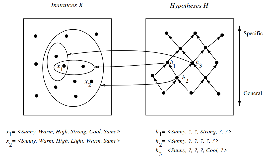
Figure 1: Instances, hypotheses, and the more_general_than relation, from Tom Mitchell Lecture 2
- Explaination of figure
- The arrows connecting hypotheses represent the more_general_than relation, with the arrow pointing toward the less general hypothesis.
- The subset of instances characterized by \(h_2\) subsumes the subset characterized by \(h_1\) hence \(h_2\) is more_general_than \(h_1\).
- \(h_2\) is more general than \(h_1\) and \(h_3\)
- Neither h1 nor h3 is more general than the other;
- although the instances satisfied by these two hypotheses intersect, neither set subsumes the other.
- \(\geq_{g}\) and \(>_{g}\) relations are defined independent of the target concept.
- They depend only on instances that satisfy the two hypotheses and not on the classification of those instances according to the target concept.
- The \(\geq_{g}\) relation defines a partial order over the hypothesis space H
- the relation is reflexive, antisymmetric, and transitive
- Partial structure because there may be pairs of hypotheses such as \(h_1\) and \(h_3\)
- \( h_1 \ngeq_{g} h_3 \)
- \( h_3 \ngeq_{g} h_1 \)
Find-S
- Finding maxmimally specific hypothesis
- Algorithm that take advantage of the above mentioned partial order to efficiently organize the search for an acceptable hypotheses that fit the training data.
- One way is to begin with the most specific possible hypothesis in H, then generalize this hypothesis each time it fails to cover an observed positive training example.
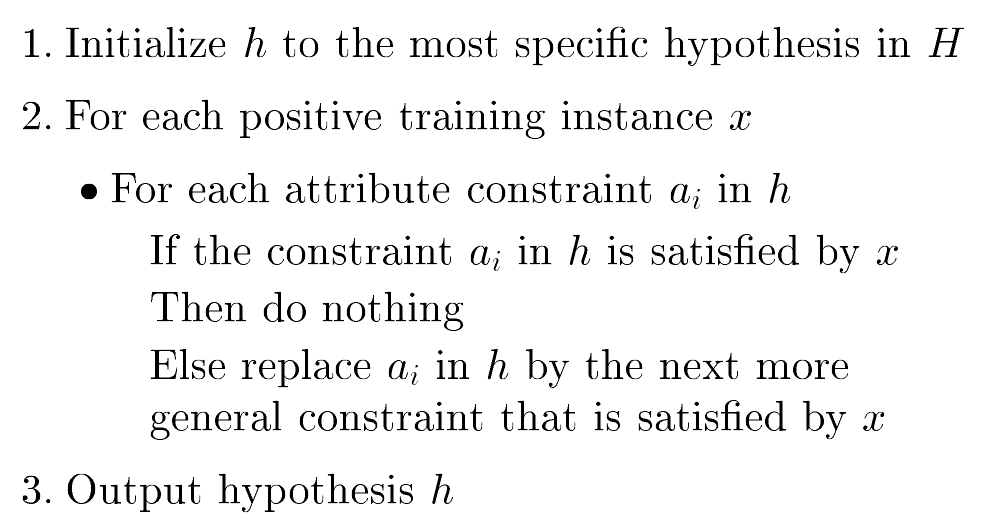
Figure 2: Find S algorithm, from Tom Mitchell Lecture 2
- Illustrating the example
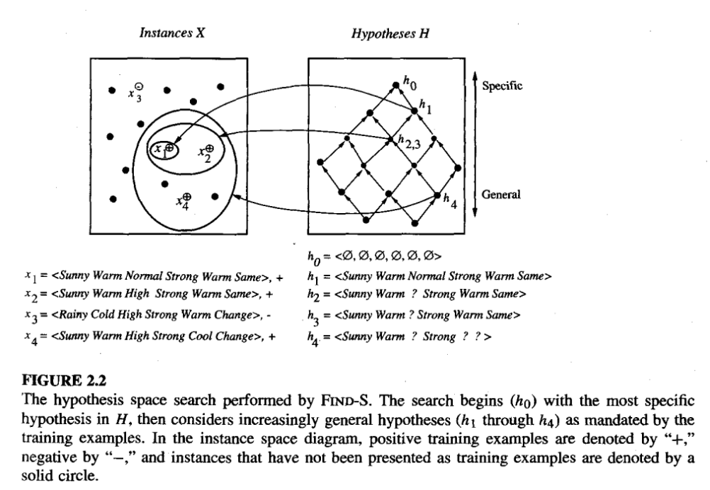
Figure 3: Find S algorithm Example, from Tom Mitchell Chapter 2
- ignores every negative examples
- The target concept c is also assumed to be in H and to be consistent with the positive training examples, c must be more_general_than_or_equal_to h. But the target concept c will never cover a negative example, thus neither will h. Therefore, no revision to h will be required in response to any negative example.
- The hypothesis is generalized only as far as necessary to cover the new positive example.
- Therefore, at each stage the hypothesis is the most specific hypothesis consistent with the training examples observed up to this point (hence the name Find-S).
- Find-S is guaranteed to output the most specific hypothesis within H that is consistent with the positive training examples.
- Its final hypothesis will also be consistent with the negative examples provided the correct target concept is contained in H, and provided the training examples are correct.
Complaints about Find-S
- Has the learner converged to the correct target concept?
- Are the training examples consistent?
- Why prefer the most specific hypothesis?
- What if there are several maximally specific consistent hypotheses?
Version Spaces and the Candidate-Elimination Algorithm
- The key idea in the Candidate-Elimination algorithm is to represent/(output a description of) the set of all hypotheses consistent with the training examples.
- Consistent Hypothesis
- A hypothesis h is consistent with a set of training examples D of target concept c if and only if \(h(x) = c(x)\) for each training example \(\langle x, c(x) \rangle\) in D.
- \( Consistent(h,D) \equiv (\forall \langle x,c(x) \rangle \in D) h(x) = c(x) \)
- x is said satisfy hypothesis when h(x) = 1, regardless of whether x is a positive or negative example of the target concept.
- However, whether x is consistent with h depends on the target concept, and in particular, whether h(x) = c(x).
Version Space
- Denoted \(VS_{H,D}\), with respect to hypothesis space H and training examples D, is the subset of hypotheses from H consistent with the training examples in D.
- \( VS_{H,D} \equiv \{ h \in H | Consistent(h, D) \} \)
The LIST-THEN-ELIMINATE Algorithm
- The algorithm first initializes the version space to contain all hypotheses in H, then eliminates any hypothesis found inconsistent with any training example.
- The version space of candidate hypotheses thus shrinks as more examples are observed, until ideally just one hypothesis remains that is consistent with all the observed examples.
- It can be the desired target concept
- If insufficient data is available to narrow the version space to a single hypothesis, then the algorithm can output the entire set of hypotheses consistent with the observed data.
- can be applied whenever the hypothesis space H is finite.
- requires exhaustively enumerating all hypotheses in H
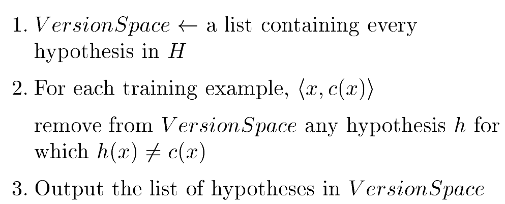
Figure 4: List-Then-Eliminate algorithm , from Tom Mitchell Chapter 2 Slides
Candidate-Elimination Learning Algorithm
It employs a much more compact representation of the version space.
In particular, the version space is represented by its most general and least general members.
Candidate_Elimination algorithm computes the version space containing all hypotheses from H that are consistent with an observed sequence of training examples.
It begins by initializing the version space to the set of all hypotheses in H ; that is, by initializing the G boundary set to contain the most general hypothesis in H,
- \( G_{0} \leftarrow \{ \langle ?, ?, ?, ?, ?, ? \rangle \} \)
- The general boundary G, with respect to hypothesis space H and training data \(D\), is the set of maximally general members of H consistent with D.
- \( G \equiv \{ g \in H|Consistent(g, D) \land (\neg \exists g’ \in H)[(g’ >_{g} g) \land Consistent(g’,D)] \} \)
and initializing the S boundary set to contain the most specific (least general)hypothesis
- \( S_{0} \leftarrow \{ \langle \emptyset, \emptyset, \emptyset, \emptyset, \emptyset, \emptyset, \rangle \} \)
- The specific boundary S, with respect to hypothesis space H and training data D, is the set of minimally general (i.e., maximally specific) members of H consistent with D.
- \( S \equiv \{ s \in H|Consistent(s, D) \land (\neg \exists s’ \in H) [ (s >_{g} s’) \land Consistent(s’,D) ] \} \)
G and S sets delimit the entire hypothesis space.
The version space is precisely the set of hypotheses contained in G, plus those contained in S plus those that lie between G and S in the partially ordered hypothesis space.
- Version space representation theorem :
- Let X be an arbitrary set of instances and let H be a set of boolean-valued hypotheses defined over X. Let c : X -> {0,1} be an arbitrary target concept defined over X, and let D be an arbitrary set of training examples {<x, c(x)>}. For all X, H, c, and D such that S and G are well defined,
- \( VS_{H,D} \equiv \{ h \in H | ( \exists s \in S ) ( \exists g \in G ) (g \geq_{g} h \geq_{g} s) \} \)
- Let X be an arbitrary set of instances and let H be a set of boolean-valued hypotheses defined over X. Let c : X -> {0,1} be an arbitrary target concept defined over X, and let D be an arbitrary set of training examples {<x, c(x)>}. For all X, H, c, and D such that S and G are well defined,
- Version space representation theorem :
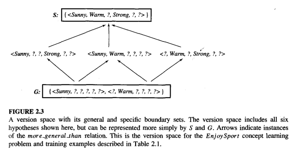
Figure 5: Version Space betn S and G, from Tom Mitchell Chapter 2
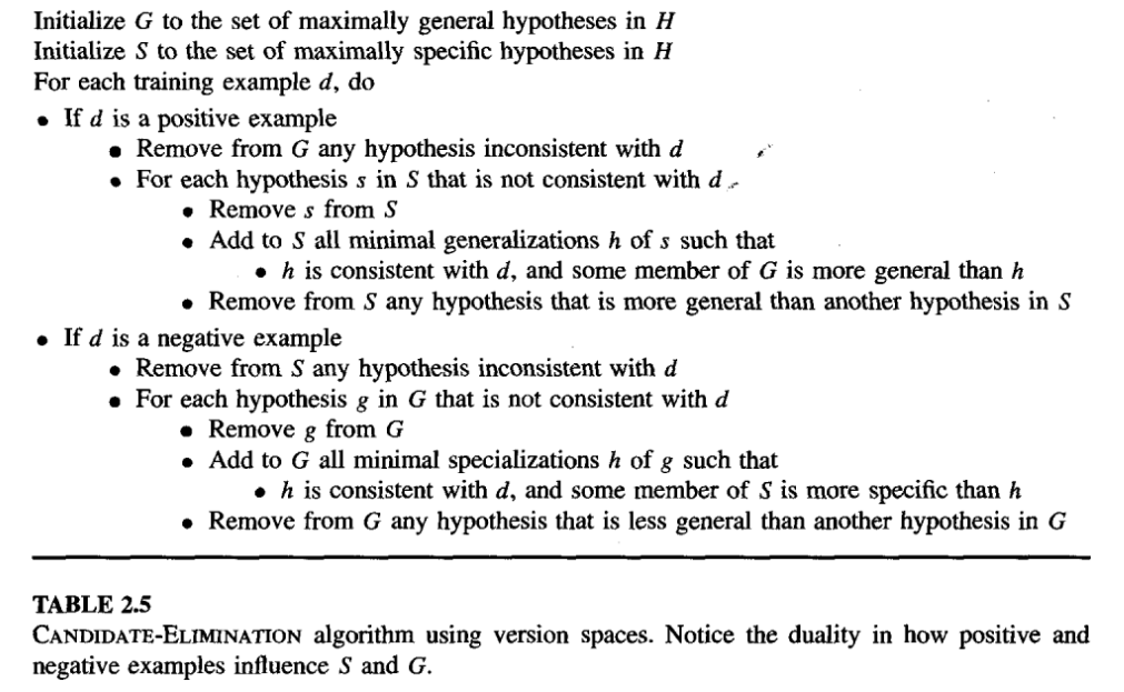
Figure 6: Candidate Elimination Algo, from Tom Mitchell Chapter 2
EnjoySport Example Using Candidate Elimination Algorithm
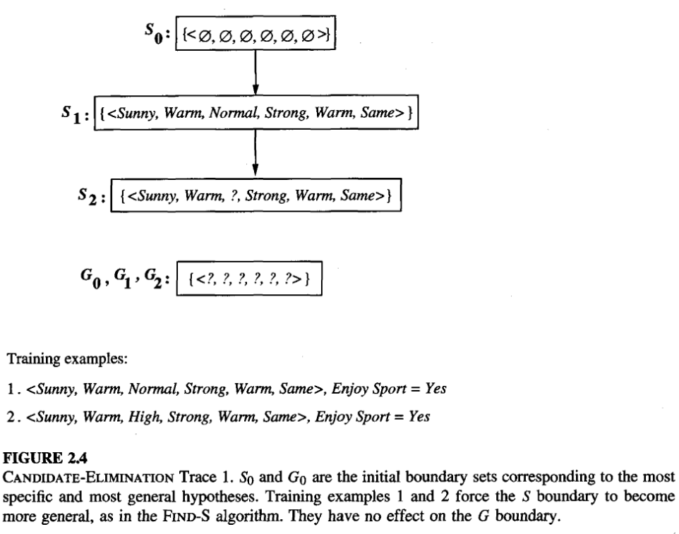
Figure 7: Candidate Elimination Trace 1, from Tom Mitchell Chapter 2
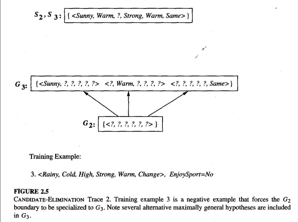
Figure 8: Candidate Elimination Trace 2, from Tom Mitchell Chapter 2
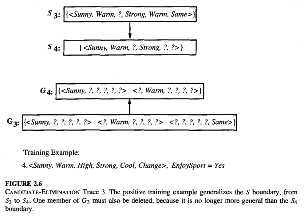
Figure 9: Candidate Elimination Trace 3, from Tom Mitchell Chapter 2
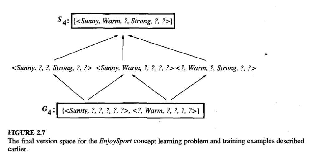
Figure 10: Final Version Space, from Tom Mitchell Chapter 2
- exclude hypothesis that is inconsistent with the previously encountered positive examples.
- Algorithm determines this simply by noting that h is not more general than the current specific boundary, [S2 in our case]
Remarks
- Candidate-Elimination Algorithm Converge to the Correct Hypothesis if,
- there are no errors in the training examples, and
- there is some hypothesis in H that correctly describes the target concept.
Candidate-Elimination algorithm’s Inductive Bias
- The target concept c is contained in the given hypothesis space H.
Fundamental questions for inductive inference
- What if the target concept is not contained in the hypothesis space?
- Can we avoid this difficulty by using a hypothesis space that includes every possible hypothesis?
- How does thes size of this hypothesis space influence the ability of the algorithm to generalize to unobserved instances?
- How does the size of the hypothesis space influence the number of training examples that must be observed?
An unbiased Learner
- The obvious solution to the question in inductive inference of assuring that the target concept is in the hypothesis space H is to provide a hypothesis space capable of representing every teachable concept.
- That is, a hypothesis space capable of representing every possible subset of the instances X.
- In general, the set of all subsets of a set X is called the power set of X,
- The number of distinct subsets that can be defined over a set X containing |X| elements (i.e., the size of the power set of X is \(2^{|X|}\).
- For enjoy sport example, attribute = 96, so \(2^{96}\) distinct target concpets.
- Reformulatin the Enjoy Sport learning task in an unbiased way by defining a new hypothesis space H’ that can represent every subset of instances;
- that is, let H’ correspond to the power set of X.
- One way to define such an H’ is to allow arbitrary disjunctions, conjunctions, and negations of our earlier hypotheses.
Inductive systems and Equivalent Deductive systems.
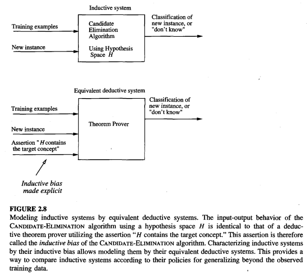
Figure 11: Modeling systems, from Tom Mitchell Chapter 2
- Inductive learners can be modelled by equivalent deductive systems
- Inductive system :
- Observe and learn from the set of instances and then draw the conclusion
- Deductive system:
- Derives conclusion and then work on it based on the previous decision
Learning algorithms from weakest to strongest bias.
- Rote-Learner:
- Learning corresponds simply to storing each observed training example in memory. Subsequent instances are classified by looking them up in memory. If the instance is found in memory, the stored classification is returned. Otherwise, the system refuses to classify the new instance.
- no inductive bias.
- Candidate-Elimination algorithm:
- New instances are classified only in the case where all members of the current version space agree on the classification. Otherwise, the system refuses to classify the new instance.
- inductive bias is that the target concept can be represented in its hypothesis space.
- Find-S:
- This algorithm, described earlier, finds the most specific hypothesisconsistent with the training examples. It then uses this hypothesis to classify all subsequent instances.
- In addition to the assumption that the target concept can be described in its hypothesis space, it has an additional inductive bias assumption: that all instances are negative instances unless the opposite is entailed by its other knowledge.